Plotting Riemann-Siegel Formula with J

The Riemann-Siegel formula, Z(t) has been used to find non-trivial zeros of Riemann's zeta function.
wikipedia

The following source code gives a numerical calculation of \[Z(t) \approx 2 \sum_{n=1}^{N}n^{-\frac{1}{2}}\cos [\theta(t) - t\log n] + R,\]

where \[\theta(t) = \Im \log \Gamma (1 + \frac{it}{2}- \frac{3}{4}) - \frac{t}{2}\log\pi . \]  This can be simplified to an easily calculatable approximation given by:
\[\theta(t) \approx \frac{t}{2}\log (\frac{t}{2\ pi}) - \frac{t}{2} - \frac{\pi}{8} + \frac{1}{48t }+ \frac{7}{5760t^{3}}.\]

The final term, [\ R,\] in the original sum, is the remainder term, which is complicated to derive but  can be reduced to a sum,[
\[ R \approx (-1)^{N-1}(\frac{t}{2 \pi})^{-1/4}[C_{0} + C_{1}(\frac{t}{2 \pi})^{-1/2} +C_{2}(\frac{t}{2 \pi})^{-1} +

C_{3}(\frac{t}{2 \pi})^{-3/2} + C_{4}(\frac{t}{2 \pi})^{-2}].\]

We will use this approximation in the calculation.

NB. Calculation of Z(x), estimate of zeta(x) for x = a +ib where b = 0.5  
NB. Riemann-Siegel formula. (from Riemann Zeta Function, H.M Edwards)      

load 'plot'  
load 'numeric trig'  
    
C0 =: 0.38268343236508977173, 0.43724046807752044936, 0.13237657548034352333, _0.01360502604767418865, _0.01356762197010358088, _0.00162372532314446528, 0.00029705353733379691,0.00007943300879521469, 0.00000046556124614504, _0.00000143272516309551, _0.00000010354847112314, 0.00000001235792708384, 0.00000000178810838577, _0.00000000003391414393, _0.00000000001632663392  

C1 =: 0.02682510262837535, _0.01378477342635185, _0.03849125048223508, _0.00987106629906208, 0.00331075976085840, 0.00146478085779542, 0.00001320794062488,_0.00005922748701847, _0.00000598024258537, 0.00000096413224562, 0.00000018334733722
  
C2 =: 0.005188542830293, 0.000309465838807, _0.011335941078299, 0.002233045741958,0.005196637408862, 0.000343991440762, _0.000591064842747, _0.000102299725479, 0.000020888392217,0.000005927665493, _0.000000164238384, _0.000000151611998  

C3 =: 0.0013397160907, _0.0037442151364, 0.0013303178920, 0.0022654660765,_0.0009548499998, _0.0006010038459, 0.0001012885828, 0.0000686573345, _0.0000005985366,_0.0000033316599, _0.0000002191929, 0.0000000789089, 0.0000000094147 
 
C4 =: 0.00046483389, _0.00100566074, 0.00024044856, 0.00102830861,_0.00076578609, _0.00020365286, 0.00023212290, 0.00003260215, _0.00002557905, _0.00000410746,0.00000117812, 0.00000024456  
    
pi2 =: +: o. 1  
    
theta =: 3 : 0  
assert. y > 0  
p1 =. ( * -:@:^.@:(%&pi2)) y  
p2 =. --: y  
p3 =. -(o. 1) % 8  
p4 =. 1 % (48 * y)  
p5 =. 7 % (5760 * y ^ 3)  
p1 + p2 + p3 + p4 + p5  
)  
    
summation =: 3 : 0 "1  
   
v =. >0{y  
m =. >1{y  
thetav =. theta v  
ms =. >: i. m  
cos =. 2&o.  
s =. +:@:(^&_0.5) * cos@:(thetav&-@:(v&*@:^.))  
+/ s ms  
)  
    
remainderterms =: 3 : 0  
im =. y  
v =. %: pi2 %~ y  
N =. <. v  
p =. v - N  
q =. 1 - 2 * p  
final =. 0  
   
mv0 =. +/ (({&C0) * (q&^@:+:)) i. # C0  
final =. mv0  
  
mv1 =. +/ (({&C1) * (q&^@:+:@:>:)) i. # C1  
mv1 =. mv1 * ((im % pi2) ^ _0.5)  
final =. final + mv1  
   
mv2 =. +/ (({&C2) * (q&^@:+:)) i. # C2  
mv2 =. mv2 * ((im % pi2) ^ _1)  
final =. final + mv2  
    
mv3 =. +/ (({&C3) * (q&^@:+:@:>:)) i. # C3  
final =. final + mv3  
    
mv4 =. +/ (({&C4) * (q&^@:+:)) i. # C4  
final =. final + mv4  
   
    
final * (_1 ^ <: N) * ((im % pi2) ^ _0.25)  
)  
   
    
z =: 3 : 0 "0  
im =. y  
v =. %: pi2 %~ y  
N =. <. v  
p =. v - N  
v1 =. summation im ; N  
v2 =. remainderterms im  
v1 + v2  
)     
   
x =: steps 0.1 100 3500  
plot x; z x  

Graphical plot

The lines:

 x =: steps 0.1 100 3500  
 plot x; z x  

create a plot of the function from 0.1 to 100 in 3500 steps, as shown below:

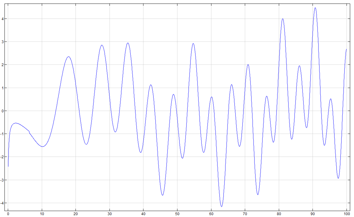
You can see the zeros of the Zeta Function from this graph. The first zero is at about x = 14.29.

Plotting Zeta function on the complex plane

 zeta3d =: 3 : 0  
 if. (0{+.y) > 0.5 do.  
 I =. >: i. 100  
 +/I^-y  
 elseif. (0{+.y) < 0.5 do.  
 z =. zeta3d 1-y  
 g =. ! 1-y  
 s =. 1 o. -:(o.1)*y  
 c =. ((o.1)^(y-1))*2^y  
 r=.z*g*s*c  
 if. 40 < |r do.  
 r =. 40  
 end.  
 r  
 elseif. 1 do.  
 0  
 end.  
 )  
   
 absz =: |@:zeta3d  
 realz=: 0&{@:+.@:zeta3d  
 imz=: 1&{@:+.@:zeta3d  
 D =.steps _15 15 40  
 'surface; viewpoint 1 _1 2' plot imz"0 j./~ D NB. use realz for real graph.

Here is a plot of the imaginary parts:

....and the real parts.

Constructing Steiner Triple Systems with OCaml

A steiner system, S(a,b,c), where a,b,c are all positive integers with a <= b <= c, is defined as a set of c elements, a collection of subsets of this set, each of size b, such that every a elements exist in exactly one subset.

e.g. S(2,3,7)

We need a set of 7 elements,

S = {0,1,2,3,4,5,6},

and we need to create subsets of S, each of size 3, where each pair of elements exist in exactly one subset:

b1 = {0,1,2}

b2 = {0,3,4}

b3 = {0,5,6}

b4 = {1,4,5}

b5 = {1,3,6}

b6 = {2,4,6}

b7 = {2,3,5}

From observation, it is clear that any two elements exist in exactly one subset b1,...,b7. We shall refer to each subset as a block.

Clearly, a steiner system does not necessarily exist for any given a,b,c. For example, there is no S(2,7,8) system. You cannot generate subsets of {0,1,2,3,4,5,6,7}, each of size 7, such that any two elements are in exactly one subset.

An S(a,b,c) is called a steiner triple system if a = 2, b = 3, and can be denoted STS(n). It can be easily proven that a S(2,3,n) exists for any n such that

\[n\cong1,3\mod6\]
But, this fact doesn't actually give us the triples of the STS(n), which is what we are interested in. The above example's 7 blocks were found by trial and error, and this isn't really a scalable method for constructing triple systems. It is not immediately clear how we can construct an STS(n) for a given n. This post creates the algorithm(s) necessary to create a STS(n) for an any applicable n.

The algorithm
We first split the problem into two parts. We will solve the problem for the case of \(n\cong 1\mod 6\) and \(n\cong3\mod6\) separately.

Case 1: \[ n\cong3\mod6\] . This is sometimes known as the Bose Construction. I won't go into details but will just present the OCaml source code, as it is not particularly long or complicated:

 let construct_for_residue_3 v =  
     let res = (v - 3) / 6 in  
     let arr = ref [] in  
     let sz = (2*res) + 1 in  
     let mult = (sz + 1) / 2 in  
     for i = 0 to sz - 1 do  
         arr := (List.append (!arr) [[[i;0];[i;1];[i;2]]])  
     done;  
     for j = 0 to sz - 2 do  
         for k = (j+1) to sz - 1 do  
             arr := (List.append (!arr) [[[j;0];[k;0];[(mult*(j + k)) mod sz; 1]];  
                             [[j;1];[k;1];[(mult*(j+k)) mod sz; 2]];  
                             [[j;2];[k;2];[(mult*(j+k)) mod sz; 0]]])  
         done  
     done;  
     !arr  

As an example,  let's try it for the case where n = 9.

 let l = construct_for_residue_3 9;;  

which gives

 [[[0; 0]; [0; 1]; [0; 2]]; [[1; 0]; [1; 1]; [1; 2]]; [[2; 0]; [2; 1]; [2; 2]];                         [[0; 0]; [1; 0]; [2; 1]]; [[0; 1]; [1; 1]; [2; 2]]; [[0; 2]; [1; 2]; [2; 0]];                         
   [[0; 0]; [2; 0]; [1; 1]]; [[0; 1]; [2; 1]; [1; 2]]; [[0; 2]; [2; 2]; [1; 0]];   
   [[1; 0]; [2; 0]; [0; 1]]; [[1; 1]; [2; 1]; [0; 2]]; [[1; 2]; [2; 2]; [0; 0]]]  

We have a List of 12 elements, where each element contains 3 sublists of ordered number pairs. e.g. the first element is

[[0; 0]; [0; 1]; [0; 2]];

Note that any two number pairs [i; j], [k;l] (where i,k is in range [0,2] and j,l is in range [0,2]),  exist in exactly one sublist.

Case 2:\(n\cong1\mod6\)
This case is slightly more complicated, but the approach is the same. The source code is given below:

 let construct_for_residue_1 v =  
     let res = (v - 1) / 6 in  
     let arr = ref [] in  
     for i = 0 to res - 1 do  
         arr := (List.append (!arr) [[[i;0];[i;1];[i;2]]])  
     done;  
     for j = 0 to 2 * res - 2 do  
         for k = j + 1 to 2 * res - 1 do  
             let z = qgf j k (2 * res) in  
             arr := (List.append (!arr) [[[j;0];[k;0];[z;1]];  
                             [[j;1];[k;1];[z;2]];  
                             [[j;2];[k;2];[z;0]]])  
         done;  
     done;  
     for l = 0 to res - 1 do  
         arr := (List.append (!arr) [[[(-1);(-1)];[l+res;0];[l;1]];  
                         [[(-1);(-1)];[l+res;1];[l;2]];  
                         [[(-1);(-1)];[l+res;2];[l;0]]])  
     done;  
     !arr  

Here, the [i,j] pairs range over different integer values but the triples are the same, i.e. a triple contains three [i,j] pairs. And every two pairs exist in exactly one triple.

For example lets try it with n = 7.

 let l = construct_for_residue_1 7;;  

This gives

  [[[0; 0]; [0; 1]; [0; 2]]; [[0; 0]; [1; 0]; [1; 1]]; [[0; 1]; [1; 1]; [1; 2]];

  [[0; 2]; [1; 2]; [1; 0]]; [[-1; -1]; [1; 0]; [0; 1]]; [[-1; -1]; [1; 1]; [0; 2]];                       
   [[-1; -1]; [1; 2]; [0; 0]]]  

Here, we can see 7 triples and it is easy to check any [[i;j];[k;l]] pair exists in one triple. We can map pairs to the b's in the example at the top of the page. For example

[0;0] ->   b1
[0;1] ->   b2
[0;2] ->   b3
[1;0] ->   b4
[1;1] ->   b5
[1;2] ->   b6
[-1;-1] -> b7

A good question at this point might be, "What's the point in this?", to which the answer is that steiner systems and combinatorial designs in general, have a wide range of connections to different areas of mathematics -  for example:

Projective and Affine Geometry (in fact the above STS(7) steiner system can be considered a projective plane);

Coding theory (e.g. Golay codes);

Group theory (Not going to go into it here, but the above STS(7) has 168 symmetries, and its group of
symmetries is isomorphic to PGL(3,2));

Experimental designs.

It's also worth noting that there are many more interesting steiner systems, beyond the triple system examples here. Probably the most noteworthy is S(5,8,24). Just a quick recap on what that means: 24 points, grouped into subsets, each of size 8, such that any given 5 points exist in exactly 1 subset. That's the definition, but the interesting point is that this object is immensely symmetric, and has over 140 million symmetries, and what's more, any 5 points can be mapped on to any other five points and still preserve symmetry.

source:

1:  (* steiner triple systems *)  
2:  open Core.Std  
3:  exception Impossible_construction  
4:    
5:    
6:  (* construct STS for vertex size 3 modulo 6 *)  
7:  let construct_for_residue_3 v =  
8:      let res = (v - 3) / 6 in  
9:      let arr = ref [] in  
10:      for i = 1 to (2 * res + 1) do  
11:          arr := (List.append (!arr) [[[i;0];[i;1];[i;2]]])  
12:      done;  
13:        
14:      for j = 1 to (2 * res + 1) do  
15:          for k = (j+1) to (2 * res + 1) do  
16:              arr := (List.append (!arr) [[[j;1];[k;1];[(j + k) / 2; 1]];  
17:                              [[j;2];[k;2];[(j+k) / 2; 2]];  
18:                              [[j;0];[k;0];[(j+k) / 2;0]]])  
19:          done  
20:      done;  
21:      !arr  
22:    
23:  (* quasigroup function -- just a function used for Skolem's construction *)  
24:  let qgf left right max =  
25:      let z = (left + right) mod max in  
26:      if z mod 2 = 0 then  
27:          z / 2  
28:      else  
29:          (z + max - 1) / 2  
30:    
31:  (* Skolem's construction - for vertex size 1 modulo 6 *)  
32:  let construct_for_residue_1 v =  
33:      let res = (v - 1) / 6 in  
34:      let arr = ref [] in  
35:      for i = 0 to res - 1 do  
36:          arr := (List.append (!arr) [[[i;0];[i;1];[i;2]]])  
37:      done;  
38:    
39:      for j = 0 to 2 * res - 2 do  
40:          for k = j + 1 to 2 * res - 1 do  
41:              let z = qgf j k (2 * res) in  
42:              arr := (List.append (!arr) [[[j;0];[k;0];[z;1]];  
43:                              [[j;1];[k;1];[z;2]];  
44:                              [[j;2];[k;2];[z;0]]])  
45:          done;  
46:      done;  
47:    
48:      for l = 0 to res - 1 do  
49:          arr := (List.append (!arr) [[[(-1);(-1)];[l+res;0];[l;1]];  
50:                          [[(-1);(-1)];[l+res;1];[l;2]];  
51:                          [[(-1);(-1)];[l+res;2];[l;0]]])  
52:      done;  
53:    
54:      !arr  
55:    
56:  (* find all blocks intersecting the element *)  
57:  let filter_element triplesystem e =  
58:      List.filter triplesystem (fun i -> List.mem i e)